
How to Create your first Pivot Tables in 5 minutes (or less!)
Pivot tables are one of the most notable features of Microsoft Excel. And it’s easy to see why once you are familiar with the feature. To a beginner, they may seem a bit mysterious or intimidating. But once you learn a few basics to get started, you will be well on your way to visualizing your data in new and useful ways.
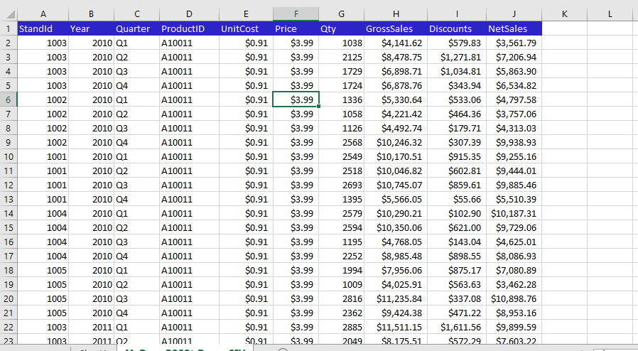
First things first, let’s start with some data. Let’s imagine we own a hot dog stand business in the big city. We have several years of sales data across several different hot dog stands, and we want to see what kind of insights a pivot table can give us.
This is the first point to note about pivot tables. The more data you have, the more pivot tables show their value. Imagine filtering on large data sets. And we all know how cumbersome such an undertaking becomes as the amount of data grows.
STEP 1: Insert your pivot table
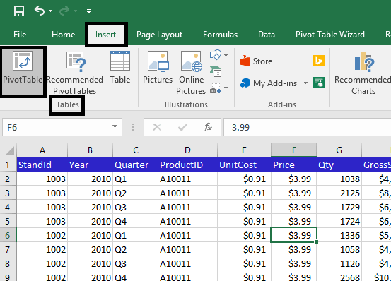
The first thing you need to do is just click into a cell within your data. Then, on the Insert tab in the ribbon, click on Pivot Table in the Tables group.
When the Create Pivot Table dialog opens, note that your data range is pre-selected. This is because we had clicked on a cell in the range of data prior to inserting our pivot table. This is a shortcut worth remembering.
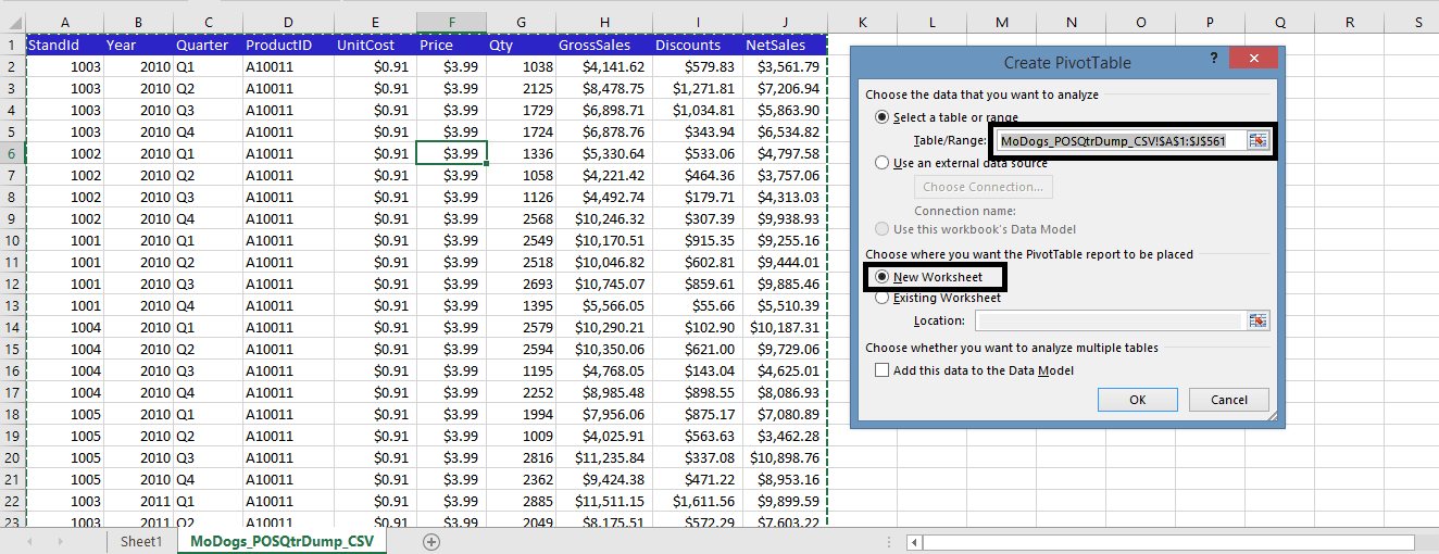
For the purposed of our example here, we will go ahead and choose a new worksheet for the placement of our pivot table. Click OK. You will now have a blank pivot table ready for you to start visualizing your data however you like.
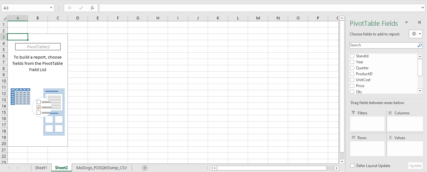
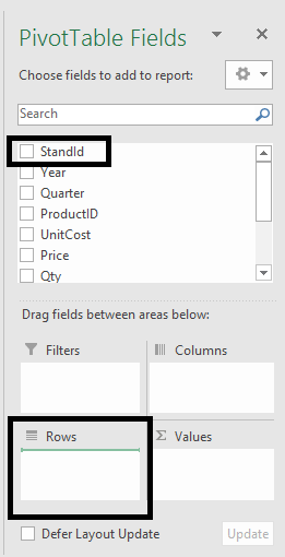
Notice your pivot table area on the left side of the worksheet and the Pivot Table Fields field list on the right side.
STEP 2: Arrange your pivot table fields
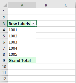
Now you need to pull in your data points according to how you would like to visualize your data. We will start by looking at each hot dog stand as a row. To do this, we will drag and drop StandId from the Field List to the Rows area.
Now we can see our pivot table taking a bit of shape.
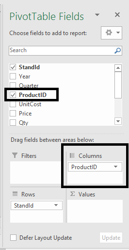
The next thing we want to do is to view our sales data by Product ID for each stand. We do this by dragging the ProductID from the Field List and dropping it into the Columns area.
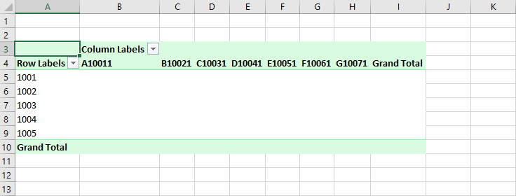
Now we have columns in addition to our rows.
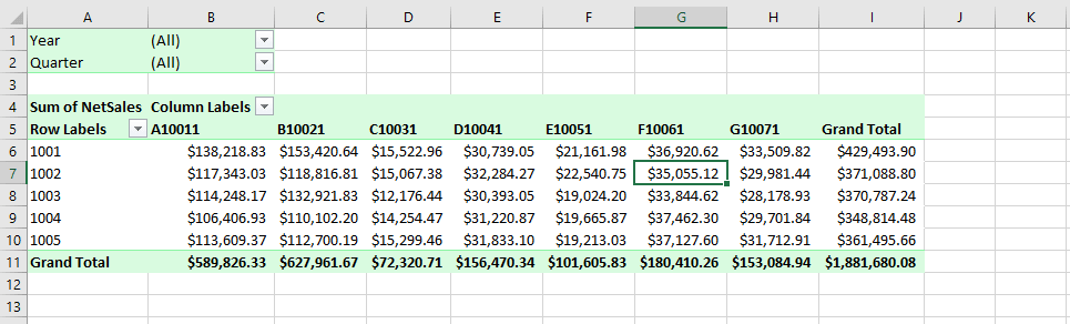
The third step to bringing our pivot table together into something meaningful is to now select the data we want to view as a cross tab of stands and sales. To do this, we simply drag and drop Net Sales to the Values area.
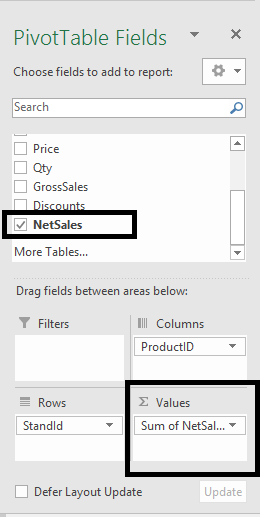
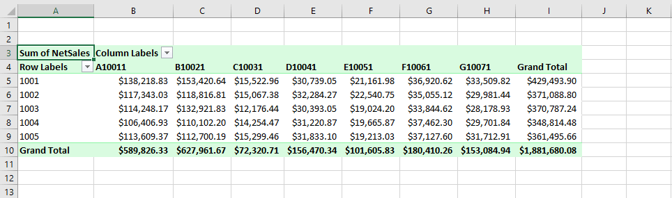
Now our pivot table shows us Net Sales by StandID by Product ID.
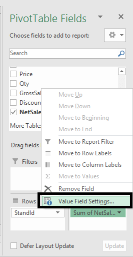
One thing to note about the Values area is that there are several value field setting available. Sum is usually the default when you drop a field to the Values area. But if you left click the field in the Value area, you can then click on Value Field Settings to open the dialog box.
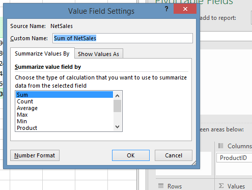
This is where you can change the value field to be summarized in different ways shown in the Summarize Values By tab of the dialog box.
Step 3: Insert our filters
We could stop right here, but since our data gives us so much we can pull in a couple of filters for additional flexibility in visualizing our Net Sales figures. We will now drag and drop both Year and Quarter to our Filters area.
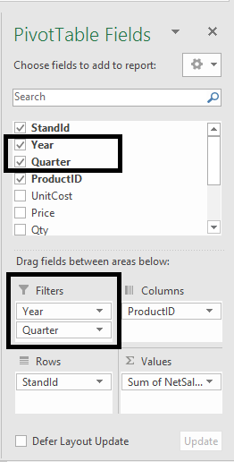
Now we notice that there are also a couple of new elements in the pivot table itself.
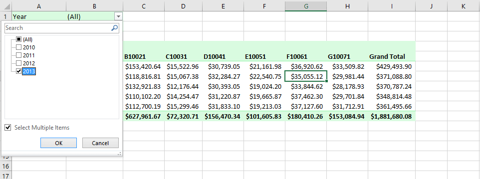
Now we can filter on a single or multiple years if we want to.
We can do the same for quarter as well. Let’s filter on 2013 Q1.
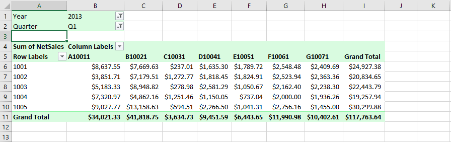
This is just a start. You could easily begin to pull in different data points to different pivot table areas to get a different perspective on your data. For a more in depth guide on how to use pivot tables, visit http://spreadsheeto.com/pivot-tables/.
FINAL THOUGHTS
In just a few short strokes of your mouse, you can generate a pivot table just like this to allow you to begin to visualize your data in ways not possible otherwise. One of the most fundamental BI tools available, pivot tables are indispensable in the Excel arsenal of capabilities for any professional.
The tutorial was written by Hannah Sharron from Spreadsheeto – feel free to reach out to her anytime at: hannah@spreadsheeto.com