Achieving Optimal Use of Shelf Space through Linear Programming

Your Product Sales is Affected by Shelf Space?

Did you notice that every time you go to a supermarket to buy something, you notice the middle shelf before the top and bottom shelves. This is contradictory to the typical sequential behavior where we like to start from one end and end at another. Of course, many a times we start from one end of the market and go around to the other end but each time we start from one of the shelves which usually is the middle one.

Does this mean that keeping a product on the middle shelf will catch more eyeballs and convert to more sales? Yes, that’s why items in a retail store are placed in a certain order no matter which store you go. This is chosen carefully based on demand and popularity of the items. With cut – throat competition going on between giants such as Walmart and target, looking into every possibility to maximize the sales involves the crucial task of shelf arrangement as one of the first tasks.

With increasing data and lots of new stores opening up every now and then, we have terabytes and petabytes of data available to process and decide the marketing strategy of every brand.

 

Where to Start From? Optimization!

Shelf space is a problem of optimization. The complexity that appears to be present for shelf space allocation can be greatly reduced by optimization. We can optimize only when there are constraints to a problem and shelf space has constraints in abundance. This includes shelf space along with size of each item, the number of shelves, number of aisles, different kinds of products, etc. For those who are unaware, optimization is a set of techniques that focuses on finding the best solution to a problem when there are constraints. Examples of optimization include deciding on the right path among a number of paths from one place to another or budgeting your monthly budget in bills, expenses and savings. In this scenario, we will deploy the concepts of linear programming and apply optimization over it to make the process simple. Let’s understand linear programming and get started with it.

 

Understand and Kick-start Linear Programming

Linear programming is a way to use mathematical concepts and programming to solve a problem, usually maximizing or minimizing using variables which exhibit linear relationship with our target. Coupled with optimization techniques and corresponding constraints, we call it linear optimization. The elements of of linear programming include the target variable to minimize or maximize, the set of linear variables which we change to optimize our target variable and our objective function which defines the connection we want between the linear variables and target variable. This is the basic concept of linear programming. We use methods such as simplex technique to solve linear programming.

 

First we need to understand the data which will be required for linear programming to solve shelf space optimization. While we can look at data in different ways to solve the same problem of shelf optimization, we will look at an intuitive and simple toy version. We won’t be dealing with the space and divide it by size dimensions. We will look at data for overall items of every product on the shelf.

 

I created a sample data using random numbers for 8 products and 8 shelf spaces. Let’s say the data comes out to be this:

 

P.1    P.2    P.3    P.4    P.5    P.6    P.7    P.8
Shelf 1    992    753    583    694    593    167    29    584
Shelf 2    65    156    622    378    788    844    837    840
Shelf 3    147    42    266    696    553    912    212    930
Shelf 4    336    731    265    826    345    155    163    813
Shelf 5    802    50    176    590    602    313    975    725
Shelf 6    215    47    293    179    904    745    35    853
Shelf 7    142    966    761    32    640    361    172    407
Shelf 8    977    774    197    637    977    420    59    306

 

It is hard to understand which product should go into which shelf just from this data to get maximum sales. These numbers can represent either sales of the products or gain in sales but whichever you take, the answer and process will remain the same. Let’s follow the concepts of linear programming and optimization to arrive at a solution.

 

First, we will define the elements of linear programming: the set of decision variables is the decision whether the product should be kept in a particular shelf or not. This means we will take a matrix of the same size (8*8 here) and multiply it with this sales matrix to get the target value. We need to maximize this value as much as possible. Thus, we will initially start with a matrix of all zeros. The values can only be 0 and 1 and will be changed by linear programming. This will be subject to some constraints. Let’s say that we cannot keep more than one product on one shelf. This means that the sum of any row in 0-1 matrix cannot be more than 1. We cannot have the same product in all the shelves. Since we have 8 shelves and 8 products, we can keep the constraint that one product can only be kept on one shelf so that all products are placed. Let’s optimize the problem now. We will use excel to get an initial solution

 

Toy Example using Excel

In excel, we need to have data as well as constraints defined in separate cells. I have done this in the excel sheet and it is available separately. Linear programming is available as an add – in named solver. One can activate it by going to File -> Options -> then Add – Ins and managing them to check Solver add – in. Solver appears in the rightmost ribbon on data tab.

Solver will show up a dialog box and we need to fill all the fields before solving. Our objective function will be to maximize the sum of the matrix multiplication of sales – matrix and 0-1 matrix. This can be achieved by using sumproduct of the two matrices. We will select solver and select the target cell. The cells to be changed is the entire 0-1 matrix. We will then add the constraints as the two constraint rows to be less than or equal to 1. Finally, we will select the solving technique as simplex. These settings should look like this:

 

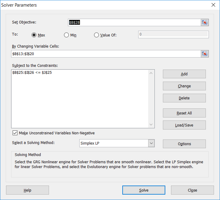
Selecting solve will quickly find out a solution to the problem. Notice that the solver tries to keep each product in the shelf which gives it the maximum sales but cannot do so for all products. If there are two products which have maximum sales for the same shelf, it will select the one which has higher sales. This toy example is relatively easy and gives the sales to be 7123 on solution. In real life, the number of shelves and products are not equal and products can also be kept on multiple shelves. Moreover, their sales on different shelves are not random numbers but have a trend based on the shelf. These complexities might not be solvable by excel alone. This is why programming languages come in handy.

R for Rescue

We have already defined the parameters for the above problem. We will use the lpSolve package in R to get our results. (link: https://cran.r-project.org/web/packages/lpSolve/lpSolve.pdf)

The package has lp.assign() function which can calculate the target based on whether we want to maximize or minimize the value assuming that we are using a 0-1 matrix. This type of problem is also known as an assignment problem.

As inputs, we only need to supply the sales matrix and the maximize/minimize parameter.

Let’s begin by reading the data.

#Reading the excel file
library(readxl)
input_data <- read_excel("input data.xlsx")
#Select the sales matrix only
Sales=input_data[1:8,2:9]
Sales.mat=as.matrix(Sales)

We do not need the shelf numbers in R. Hence we have removed it. This matrix is now passed into lp.assign package

#Using lpSolve package
#install.packages("lpSolve")
library(lpSolve)
result=lp.assign(Sales.mat,direction = "max")

Result contains the solution matrix as well as our final target value. We can access them by using the objval and Solution lists in result.

#Fetching the target value
result$objval
7123
#Getting the solution matrix
result$solution
[,1] [,2] [,3] [,4] [,5] [,6] [,7] [,8]
[1,]    1    0    0    0    0    0    0    0
[2,]    0    0    1    0    0    0    0    0
[3,]    0    0    0    0    0    1    0    0
[4,]    0    0    0    1    0    0    0    0
[5,]    0    0    0    0    0    0    1    0
[6,]    0    0    0    0    0    0    0    1
[7,]    0    1    0    0    0    0    0    0
[8,]    0    0    0    0    1    0    0    0

This is the same 0-1 matrix that we optimized in excel.

Conclusion : It’s More Difficult Than It Looks

Even though it looked pretty and simple in R and excel but it is much more difficult. At certain times, a single solution is not possible and both solver and R yield different results due to many local optima. The problems are so complex that we can’t accurately visualize the problem, much less find a way to solve it quickly so there are many intermediate solutions which are given out by excel or R. These solutions differ based on what starting values we started with. For example, we started with a matrix of all zeros in this problem. Since this problem was simple and had only one solution, we will get the same results no matter what starting values we took. However, in some cases, our starting can help reach better local solutions.

 

The problems become even more complex and slower when the constraints are loose. In this example, we worked with very narrow constraints so the only possible values for each cell were either 0 or 1. Even so, with an 8*8 matrix, there were 64 cells having 2 values or 2^64 possible combinations which are greatly reduced by constraints (8! =40,320 In this case). This is why constraints play an important role in problem optimization and reducing the number of possibilities. Certain products may have a special requirements or may be essential to a market. Say for example, if business says that one of the products is a beverage and should only be kept in shelf 3 as it is the refrigerator, our problem instantly reduces from 8*8 to 7*7 matrix. Thus, it is good to evaluate products and apply more knowledge than taking them invariantly. One such method is to classify products based on their types and dividing them into different aisles. One can have a different aisle for beverages and products which require a cold environment. All biscuits can be kept separately and so as all spices, groceries, utensils and so on. It depends on how your business sees the problem of shelf space optimization.

 

While it is not possible to solve every type of problem, there are certainly tips which help make a solution better in case of linear programming. The first step is understanding the problem from the perspective of implementation. One should know how the products are and their maintenance when they are placed in a store. Some may require a cool environment while others may have a short shelf life and need to be sold quickly or losses will be incurred. Those goods which should have a higher sales can be kept closer to the store entrance and the purchase counter so that customers see it as soon as they enter or while they are waiting in line. Some products may be delicate or cannot be carried easily such as heavy flour packets or oil packages. It is important that they are kept with care. If oil is spilt, it might make other products bad or be a cause of fire. Such products can be kept separately. It is also important to know the design of your store. Different types of products can be kept in different sections and managed together. Types of products can then be further studied to know how the sections should be arranged to get maximum sales from each section. Similarly, shelf height is another factor to consider so that one understands that products of large height cannot be kept in some places or heavy products cannot be kept on top shelves or they may result in injuries. All such constraints can be applied to simplify problems and achieve the best possible outcome.

 

The entire R code used in this article is given below:

#Reading the excel file
library(readxl)
input_data <- read_excel("input data.xlsx")
#Select the sales matrix only
Sales=input_data[1:8,2:9]
Sales.mat=as.matrix(Sales)
#Using lpSolve package
#install.packages("lpSolve")
library(lpSolve)
result=lp.assign(Sales.mat,direction = "max")
#Fetching the target value
result$objval
#Getting the solution matrix
result$solution

Author Bio

This article was contributed by Perceptive Analytics. Madhur Modi, Jyothirmai Thondamallu, Saneesh Veetil and Chaitanya Sagar contributed to this article.

Perceptive Analytics provides Tableau Consulting, data analytics, business intelligence and reporting services to e-commerce, retail, healthcare and pharmaceutical industries. Our client roster includes Fortune 500 and NYSE listed companies in the USA and India.