
Association Rules in R
“Association rules are if/then statements for discovering interesting relationships between seemingly unrelated data in a large databases or other information repository.”
Association rules are used extensively in finding out regularities between products bought at supermarkets. An example of an association rule would be “If a customer buys a loaf of bread, he is 70% likely to also purchase cheese.”
So, what is a rule?
A rule is a basic notation that represents which item or items is frequently bought with what other item or items. An association rule has two parts, a LHS and a RHS. Below is a representation of this rule.
itemset A => itemset B or
{bread, eggs} => {milk}
This means, the item or items on the right were frequently purchased along with item or items on the left. Association rules are used for many activities such as –
- Product pricing
- Product placement
- Web Usage mining
- Intrusion detection
- Market basket analysis
How to Measure the Strength of a Rule?
Now that we know what a rules are, the next question that pops up is “How do we measure the strength of a rule?”
The three main measures to decide the strength of a rule are –
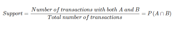
Support
Which basically means, support is calculated by dividing the number of transactions with both A and B by the total number of transitions.
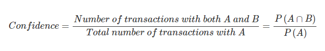
Confidence
It signifies the likelihood of item B being purchased when item A is purchased
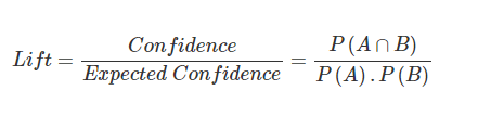
Lift
Lift signifies the likelihood of item B being purchased when item A is purchased while taking into account the popularity of. As lift increases, the chances of A and B occurring together also increases.
Apriori Algorithm
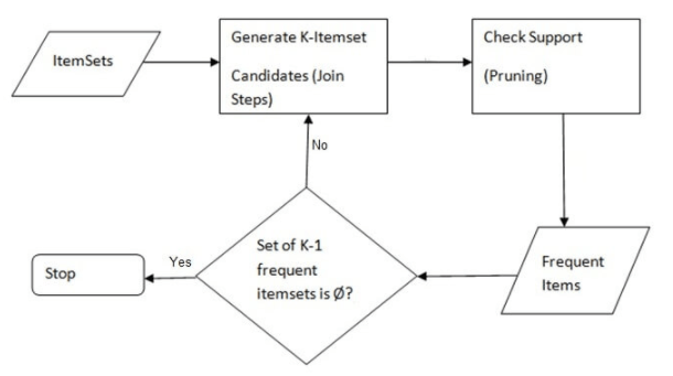
The Apriori algorithm is used to find the rules that we discussed above. The algorithm works by employing an iterative approach. This is known as level-wise search, where k-itemsets are used to explore k+1 itemsets.
- First step involves generating frequent itemsets of length one. This is repeated until no new frequent itemsets can be identified
- Next, start generating length k+1 candidates from length k frequent itemsets
- Next step is to prune the candidate itemsets containing subsets of length k that are infrequent
- Count the support of each candidate by scanning the DB
- Eliminate candidates that are infrequent, leaving only those that are frequent
Below is a flowchart of the above mentioned steps –
Case Study
Let’s look at some data that has been generated from a supermarket POS (point of sale). You can download it from here or load the ‘Groceries’ dataset from arules package in R. The one difference between these methods is that the data in the arules package is already in the form of a sparse matrix. Whereas the downloaded data is in the below mentioned format.
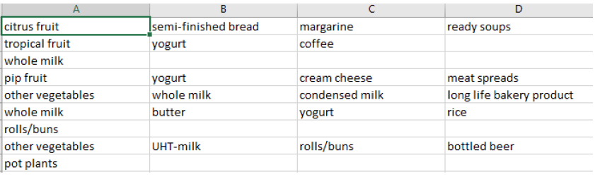
As seen from the above picture, each row is a transaction. The first transaction contains –
- Citrus fruit
- Semi-finished bread
- Margarine
- Ready soups
This data needs to be converted into a sparse matrix of sorts as shown below.
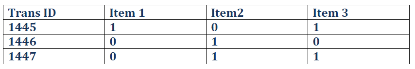
In the above table, each row represents a transaction. And each column represents an item. If there is a transaction which involves an item that particular cell shall be represented with a 1 if not 0 is put in its place.
So, let’s start off by calling the libraries required to perform market basket analysis
>require(arules)
Loading required package: arules
Loading required package: Matrix
Attaching package: �arules�
The following objects are masked from �package:base�:
abbreviate, write
>require(arulesViz)
Loading required package: arulesViz
Loading required package: grid
Reading the transactional data-
>gr <-read.transactions(file.choose(), sep = ",")
Now that the data has been loaded. Let’s look at the summary of the data.
>summary(gr)
transactions as itemMatrix in sparse format with
9835 rows (elements/itemsets/transactions) and
169 columns (items) and a density of 0.02609146
most frequent items:
whole milk other vegetables rolls/buns soda
2513 1903 1809 1715
yogurt (Other)
1372 34055
element (itemset/transaction) length distribution:
sizes
1 2 3 4 5 6 7 8 9 10 11 12 13 14 15 16
2159 1643 1299 1005 855 645 545 438 350 246 182 117 78 77 55 46
17 18 19 20 21 22 23 24 26 27 28 29 32
29 14 14 9 11 4 6 1 1 1 1 3 1
Min. 1st Qu. Median Mean 3rd Qu. Max.
1.000 2.000 3.000 4.409 6.000 32.000
includes extended item information - examples:
labels
1 abrasive cleaner
2 artif. sweetener
3 baby cosmetics
Some of the inferences that can be made from the summary is –
- There are 9835 transactions and 169 unique items
- The most frequent items are also mentioned in the summary
- The sizes displays the count for each transaction
The first few transactions can be obtained by using inspect. The first 15 transactions are –
>inspect(gr[1:15])
items
[1] {citrus fruit,
margarine,
ready soups,
semi-finished bread}
[2] {coffee,
tropical fruit,
yogurt}
[3] {whole milk}
[4] {cream cheese,
meat spreads,
pip fruit,
yogurt}
[5] {condensed milk,
long life bakery product,
other vegetables,
whole milk}
[6] {abrasive cleaner,
butter,
rice,
whole milk,
yogurt}
[7] {rolls/buns}
[8] {bottled beer,
liquor (appetizer),
other vegetables,
rolls/buns,
UHT-milk}
[9] {pot plants}
[10] {cereals,
whole milk}
[11] {bottled water,
chocolate,
other vegetables,
tropical fruit,
white bread}
[12] {bottled water,
butter,
citrus fruit,
curd,
dishes,
flour,
tropical fruit,
whole milk,
yogurt}
[13] {beef}
[14] {frankfurter,
rolls/buns,
soda}
[15] {chicken,
tropical fruit}
The frequency for any of the 169 items can obtained by using the itemfrequency command. Let’s look at the frequency of the first four items –
>itemFrequency(gr[,1:4])
abrasive cleaner artif. sweetener baby cosmetics
0.0035587189 0.0032536858 0.0006100661
baby food
0.0001016777
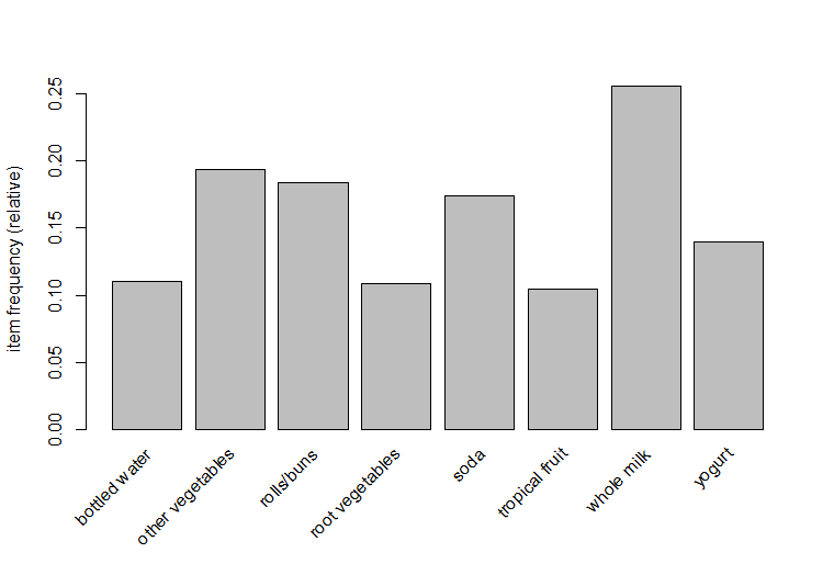
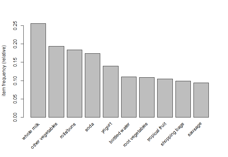
Frequency Plots
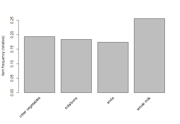
The frequencies can also be plotted. Below are some of the frequency plots for varying support values –
>itemFrequencyPlot(gr, support = .10)
>itemFrequencyPlot(gr, support = .15)
Alternatively frequency plots can be obtained for the top 10 frequently bought items –
>itemFrequencyPlot(gr,topN=10,type="absolute")

>itemFrequencyPlot(gr,topN=10,type="relative")
Defining Rules
Now that we have have an idea of how the data looks. We proceed to create rules. Rules are formed by defining the minimum support and confidence levels. Also the minlen option lets us to set the minimum number of items for both the LHS and RHS.
> rules <- apriori(gr, parameter = list(supp = 0.005, conf = 0.20, minlen =2)) Apriori Parameter specification: confidence minval smax arem aval originalSupport maxtime support minlen maxlen 0.2 0.1 1 none FALSE TRUE 5 0.005 2 10 target ext rules FALSE Algorithmic control: filter tree heap memopt load sort verbose 0.1 TRUE TRUE FALSE TRUE 2 TRUE Absolute minimum support count: 49 set item appearances ...[0 item(s)] done [0.00s]. set transactions ...[169 item(s), 9835 transaction(s)] done [0.01s]. sorting and recoding items ... [120 item(s)] done [0.00s]. creating transaction tree ... done [0.00s]. checking subsets of size 1 2 3 4 done [0.02s]. writing ... [872 rule(s)] done [0.01s]. creating S4 object ... done [0.01s]. > summary(rules)
set of 872 rules
rule length distribution (lhs + rhs):sizes
2   3   4
265 559  48
Min. 1st Qu.  Median    Mean 3rd Qu.    Max.
2.0     2.0     3.0     2.8     3.0     4.0
summary of quality measures:
support        confidence        lift         count
Min.   :0.005   Min.   :0.20   Min.   :0.9   Min.   : 50
1st Qu.:0.006   1st Qu.:0.25   1st Qu.:1.6   1st Qu.: 57
Median :0.007   Median :0.32   Median :1.9   Median : 71
Mean   :0.010   Mean   :0.35   Mean   :2.0   Mean   : 98
3rd Qu.:0.010   3rd Qu.:0.43   3rd Qu.:2.4   3rd Qu.:101
Max.   :0.075   Max.   :0.70   Max.   :4.1   Max.   :736
mining info:
data ntransactions support confidence
gr          9835   0.005        0.2
From the summary we can infer the following –
- 872 rules were formed
- Minimum and maximum values for support, confidence and lift are displayed
- Out of the 872 rules formed the counts of rule length is also displayed
Once the rules are formed, we can have a look at the some of the formed rules.
> options(digits=2)
> inspect(rules[1:10])
lhs              rhs                support confidence lift count
[1]  {cake bar}    => {whole milk}       0.0056  0.42       1.66 55
[2]  {dishes}      => {other vegetables} 0.0060  0.34       1.76 59
[3]  {dishes}      => {whole milk}       0.0053  0.30       1.18 52
[4]  {mustard}     => {whole milk}       0.0052  0.43       1.69 51
[5]  {pot plants}  => {whole milk}       0.0069  0.40       1.57 68
[6]  {chewing gum} => {soda}             0.0054  0.26       1.47 53
[7]  {chewing gum} => {whole milk}       0.0051  0.24       0.95 50
[8]  {canned fish} => {other vegetables} 0.0051  0.34       1.75 50
[9]  {pasta}       => {whole milk}       0.0061  0.41       1.59 60
[10] {herbs}       => {root vegetables}  0.0070  0.43       3.96 69
Just looking at these rules makes little sense, let’s sort the rules based on confidence levels.
> rules<-sort(rules, by="confidence", decreasing=TRUE) > options(digits=2)
> inspect(rules[1:10])
lhs                     rhs                support confidence lift count
[1]  {root vegetables,
tropical fruit,
yogurt}             => {whole milk}        0.0057       0.70  2.7    56
[2]  {other vegetables,
pip fruit,
root vegetables}    => {whole milk}        0.0055       0.68  2.6    54
[3]  {butter,
whipped/sour cream} => {whole milk}        0.0067       0.66  2.6    66
[4]  {pip fruit,
whipped/sour cream} => {whole milk}        0.0060       0.65  2.5    59
[5]  {butter,
yogurt}             => {whole milk}        0.0094       0.64  2.5    92
[6]  {butter,
root vegetables}    => {whole milk}        0.0082       0.64  2.5    81
[7]  {curd,
tropical fruit}     => {whole milk}        0.0065       0.63  2.5    64
[8]  {citrus fruit,
root vegetables,
whole milk}         => {other vegetables}  0.0058       0.63  3.3    57
[9]  {other vegetables,
pip fruit,
yogurt}             => {whole milk}        0.0051       0.62  2.4    50
[10] {domestic eggs,
pip fruit}          => {whole milk}        0.0054       0.62  2.4    53
Now things are starting to make sense, looking at the first transaction – there is a high likelihood of whole milk being purchased along with root vegetables, tropical fruit and yogurt than can other purchases. Similar to sorting rules confidence, they can also be sorted by lift levels.
> rules<-sort(rules, by="lift", decreasing=TRUE) > options(digits=2)
> inspect(rules[1:10])
lhs                     rhs                  support confidence lift count
[1]  {citrus fruit,
other vegetables,
whole milk}         => {root vegetables}     0.0058       0.45  4.1    57
[2]  {butter,
other vegetables}   => {whipped/sour cream}  0.0058       0.29  4.0    57
[3]  {herbs}              => {root vegetables}     0.0070       0.43  4.0    69
[4]  {citrus fruit,
pip fruit}          => {tropical fruit}      0.0056       0.40  3.9    55
[5]  {berries}            => {whipped/sour cream}  0.0090       0.27  3.8    89
[6]  {other vegetables,
tropical fruit,
whole milk}         => {root vegetables}     0.0070       0.41  3.8    69
[7]  {whipped/sour cream,
whole milk}         => {butter}              0.0067       0.21  3.8    66
[8]  {root vegetables,
whole milk,
yogurt}             => {tropical fruit}      0.0057       0.39  3.7    56
[9]  {other vegetables,
pip fruit,
whole milk}         => {root vegetables}     0.0055       0.41  3.7    54
[10] {citrus fruit,
tropical fruit}     => {pip fruit}           0.0056       0.28  3.7    55
A lift value greater than one indicates that items in RHS are more likely to be purchases with items on LHS. Similarly a lift value lesser than one implies that items in RHS are unlikely to be purchased with items in LHS. In the above first transaction, we can conclude that root vegetables are purchased four times more with citrus fruit, other vegetables and whole milk than it being purchased alone.
Making Product Recommendations
Now that we have figured out how to form rules and sort them. The next step is getting product recommendations, let’s look at the top product recommendations for people who purchased root vegetables. This can be accomplished by setting the LHS as root vegetables and RHS as default.
> rules <- apriori(gr, parameter = list(supp = 0.005, conf = 0.20, minlen =2), appearance = list(default="rhs",lhs="root vegetables")) Apriori Parameter specification: confidence minval smax arem aval originalSupport maxtime support minlen maxlen 0.2 0.1 1 none FALSE TRUE 5 0.005 2 10 target ext rules FALSE Algorithmic control: filter tree heap memopt load sort verbose 0.1 TRUE TRUE FALSE TRUE 2 TRUE Absolute minimum support count: 49 set item appearances ...[1 item(s)] done [0.01s]. set transactions ...[169 item(s), 9835 transaction(s)] done [0.02s]. sorting and recoding items ... [120 item(s)] done [0.00s]. creating transaction tree ... done [0.01s]. checking subsets of size 1 2 done [0.01s]. writing ... [4 rule(s)] done [0.01s]. creating S4 object ... done [0.01s]. > summary(rules)
set of 4 rules
rule length distribution (lhs + rhs):sizes
2
4
Min. 1st Qu.  Median    Mean 3rd Qu.    Max.
2       2       2       2       2       2
summary of quality measures:
support        confidence        lift          count
Min.   :0.024   Min.   :0.22   Min.   :1.21   Min.   :239
1st Qu.:0.025   1st Qu.:0.23   1st Qu.:1.58   1st Qu.:250
Median :0.037   Median :0.34   Median :1.73   Median :360
Mean   :0.037   Mean   :0.34   Mean   :1.73   Mean   :360
3rd Qu.:0.048   3rd Qu.:0.44   3rd Qu.:1.88   3rd Qu.:470
Max.   :0.049   Max.   :0.45   Max.   :2.25   Max.   :481
mining info:
data ntransactions support confidence
gr          9835   0.005        0.2
Now we sort the rules by lift.
> rules<-sort(rules, by="lift", decreasing=TRUE) > options(digits=2)
> inspect(rules)
lhs                  rhs                support confidence lift count
[1] {root vegetables} => {other vegetables} 0.047   0.43       2.2  466
[2] {root vegetables} => {whole milk}       0.049   0.45       1.8  481
[3] {root vegetables} => {yogurt}           0.026   0.24       1.7  254
[4] {root vegetables} => {rolls/buns}       0.024   0.22       1.2  239
The top product recommendation for people who purchased root vegetables are other vegetables followed by whole milk.
Conclusion
As we have discussed in the article, association rules are used extensively in a variety of fields. We have also seen how market basket analysis can done with the help of the Apriori algorithm. This is quite helpful in getting product recommendations for customers. So, go ahead and start mining your own datasets.
Author Bio:
This article was contributed by Perceptive Analytics. Rohit, Sinna Muthiah Meiyappan, Saneesh Veetil and Chaitanya Sagar contributed to this article.
Perceptive Analytics provides Tableau Consulting, data analytics, business intelligence and reporting services to e-commerce, retail, healthcare and pharmaceutical industries. Our client roster includes Fortune 500 and NYSE listed companies in the USA and India.