
Zipf’s Law and Introduction to Text Analytics
Hello Friends! recently I was doing some research and got to know about an interesting law called Zipf’s law. You can read about it on wikipedia and how it is applicable almost everywhere.
Wikipedia says- Zipf’s law states that given some corpus of natural language utterances, the frequency of any word is inversely proportional to its rank in the frequency table. Thus the most frequent word will occur approximately twice as often as the second most frequent word, three times as often as the third most frequent word, etc.: the rank-frequency distribution is an inverse relation. For example, in the Brown Corpus of American English text, the word “the” is the most frequently occurring word, and by itself accounts for nearly 7% of all word occurrences (69,971 out of slightly over 1 million). True to Zipf’s Law, the second-place word “of” accounts for slightly over 3.5% of words (36,411 occurrences), followed by “and” (28,852). Only 135 vocabulary items are needed to account for half the Brown Corpus.
I thought to make a tutorial and visualize Zipf’s Law. I think it will be good way to indroduce about the basic text analytics in R by using Zipf’s law. You can find all the sources/references in the end of the tutorial.
Below the R code you can directly copy and paste in console and start to play with it, the code is very easy to understand and properly commented. You will need few packages to install in R.
1. Install and Load Packages
# Install
install.packages("tm") # for text mining
install.packages("SnowballC") # for text stemming
install.packages("wordcloud") # word-cloud generator
install.packages("RColorBrewer") # color palettes
#Load
library("tm")
library("SnowballC")
library("wordcloud")
library("RColorBrewer")
2. Load, Transform and Clean data
#text <- readLines(file.choose())
filePath <- "https://archive.org/stream/AnneFrankTheDiaryOfAYoungGirl_201606/
Anne-Frank-The-Diary-Of-A-Young-Girl_djvu.txt"
text <- readLines(filePath)
docs <- Corpus(VectorSource(text))
#Inspect the data
#inspect(docs)
#Text transformation and cleaning like removing white spaces,numbers etc.
toSpace <- content_transformer(function (x , pattern ) gsub(pattern, " ", x))
docs <- tm_map(docs, toSpace, "/")
docs <- tm_map(docs, toSpace, "@")
docs <- tm_map(docs, toSpace, "\\|")
# Convert the text to lower case
docs <- tm_map(docs, content_transformer(tolower))
# Remove numbers
docs <- tm_map(docs, removeNumbers)
# Remove english common stopwords
#docs <- tm_map(docs, removeWords, stopwords("english"))
# Remove your own stop word. specify your stopwords as a character vector
#docs <- tm_map(docs, removeWords, c("blabla1", "blabla2"))
# Remove punctuations
docs <- tm_map(docs, removePunctuation)
# Eliminate extra white spaces
docs <- tm_map(docs, stripWhitespace)
dtm <- TermDocumentMatrix(docs)
m <- as.matrix(dtm)
v <- sort(rowSums(m),decreasing=TRUE)
d <- data.frame(word = names(v),freq=v)
#assigning the ranks
zipf<- cbind(d, Rank=1:nrow(d), per=100*d$freq/sum(d$freq))
3. Visualizing the Zipf’s law
Plot 1:
#Rank-Frequncy plot
plot(zipf$Rank,zipf$freq, xlab="Rank", ylab="Frequency",log="x")
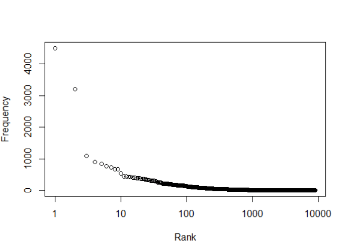
Frequncy-Rank Graph
This part of the code is to add labels to the the points(NOT recommended if you
have more than 10 points on the graph)
#to add labels
#text(zipf$Rank,zipf$freq,labels=zipf$word)
Plot 2:
#Rank-Percent Plot
plot(zipf$Rank, zipf$per,xlab="Rank", ylab="Percent", log="x")
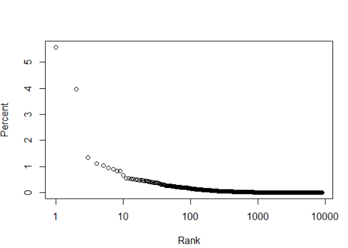
Frequncy Percent- Rank Graph
#Word Cloud
wordcloud(words = zipf$word, freq = d$freq, min.freq = 1, max.words=200,
random.order=FALSE, rot.per=0.35, colors=brewer.pal(8, "Dark2"))
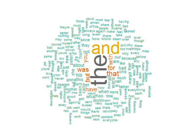
Word Cloud
As you can see the pattern is almost similar to the zipf’s law but the difference is because of the smaller data set. I couldn’t use the larger data set due to limitation of my system configurations. But the data set is big enough to introduce about the text analytics, word cloud, finding frequencies etc.
As you can see the above wordcloud doesn’t give much information about the important words in the text it is because I haven’t remove the stop words . Stop words are commonly used words like “the”,”and”,”of” etc. After removing the stop words the wordcloud will look something like this:
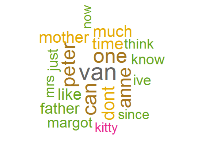
Word Cloud 2
And the beauty of the word cloud is to visualize and have a quick idea about the text. So, the input file was famous book/diary Titled “Anne Frank The Diary Of A Young Girl”. The words in word clouds are mother, father, kitty(her diary) which is obvious. Anyone can have a idea about the text by just looking at the word cloud.
Text analytics is one of the major part of modern analytics which includes NLP, Speech recognition etc. I’ll come up with few more text analytics tutorials like sentiment analysis. Till then try to explore and read more about it. I’ve mentioned sources, references and further readings.
Sources:
The Zipf Mystery (Check out the video description for awesome resources)
Word Cloud in R | Data Used
Please comment your suggestions or queries.
Thanks for reading and keep visiting Analytics Tuts for more tutorials.
Pingback: Learning 80% of Spanish in 2 months