Conditional Formatting on Errors in Excel

Hello Friends! Today we’ll be seeing a very simple and very useful way to find out the errors in Excel sheet. This is very handy if you have a sheet with 100’s of rows and columns and can save lot of time.

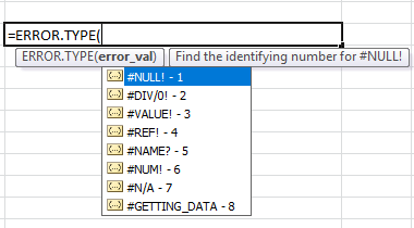
Excel considers the following 7 types of errors:

#DIV/0!
#N/A
#NAME?
#NULL!
#NUM!
#REF!
#VALUE!

You can check the error type using ERROR.TYPE() function.

 

Now let’s consider you working on Excel with some 10-15 rows and 3-4 columns contains formulas finding the errors will be very easy right?

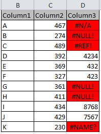
Now consider the same with 100’s of rows and columns contains formulas. How will you find if there is any error present in your Excel.

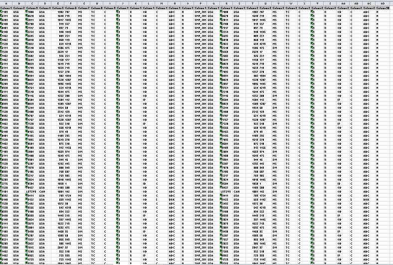
To find the errors in your Excel sheet in one shot.

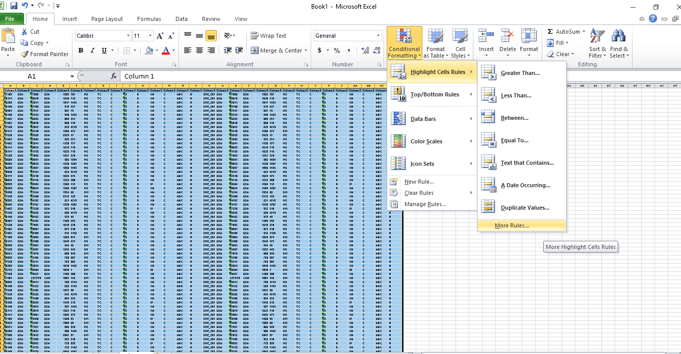
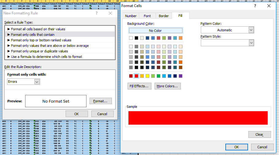
First select all the data in your sheet then go to Conditional Formatting> Highlight Cells Rules > New Rules (as shown).

Then a New Formatting Rule window will open. Select the Format only cells that contain option then from the Rule Description select Errors (as shown in the image below).Then click on format here we’ll format the cells which contains the errors. I’m selecting cell fill color as Red. Click Ok and done.

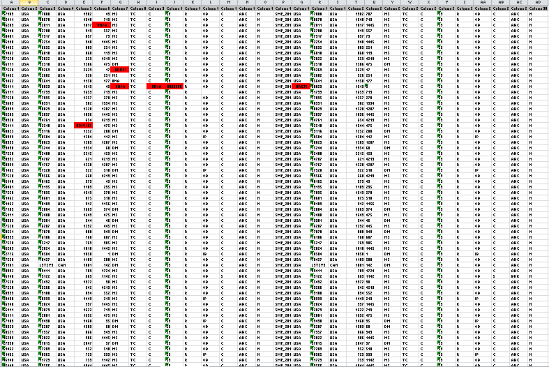
Once you press Ok, you’ll see the cells with red color if it contains Errors.

Thanks to Varun S for the trick.

Keep visiting Analytics Tuts for more tutorials.

Thanks for reading! Comment your suggestion and queries.