Pivot Tables in Excel

Today we’ll be learning about Pivot Table. Pivot Tables is one of the most powerful features of Excel. Pivots Tables are great way to summarize, analyze, explore, and present your data.
Worksheet is attached for downloading and reuse.

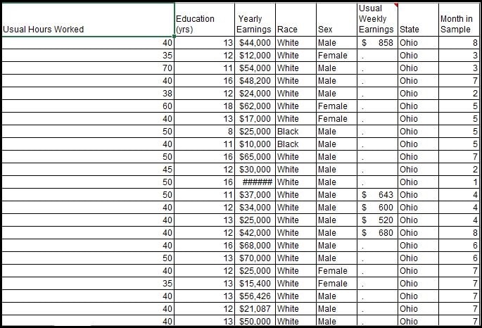
Data

The data I’ll be using contains details of 6366 full-time workers in five North-Central States, March 1999 and it looks like.

 

Creating Pivot Table

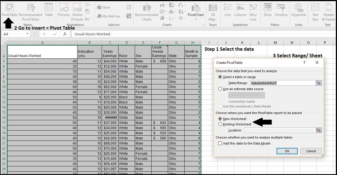
Select the data range which to be used to for pivot table.

a. Select data range
b. Go to Insert > Pivot Table
c. A window will appear asking for range and other option.

 

Working with Pivot Table

A New sheet will be added which contains a Pivot Table. In right side you’ll see the PivotTable Fields area.

Drag Education to Rows and Yearly Earnings to Values to create basic Pivot Table.

 

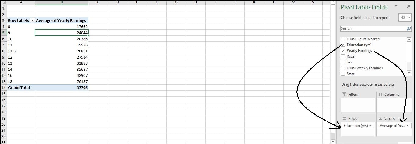
Area Fields can be explained as follows:

 

Change Calculation and Number Format

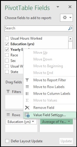
Click on the drop-down menu in Values (here Average of Yearly Earnings) and click Value Field Settings.

 

A window will appear where you can change your Column name and calculation (Sum,Average,Count etc.)

 

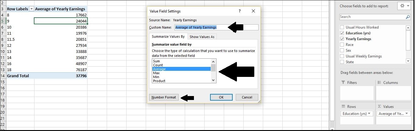
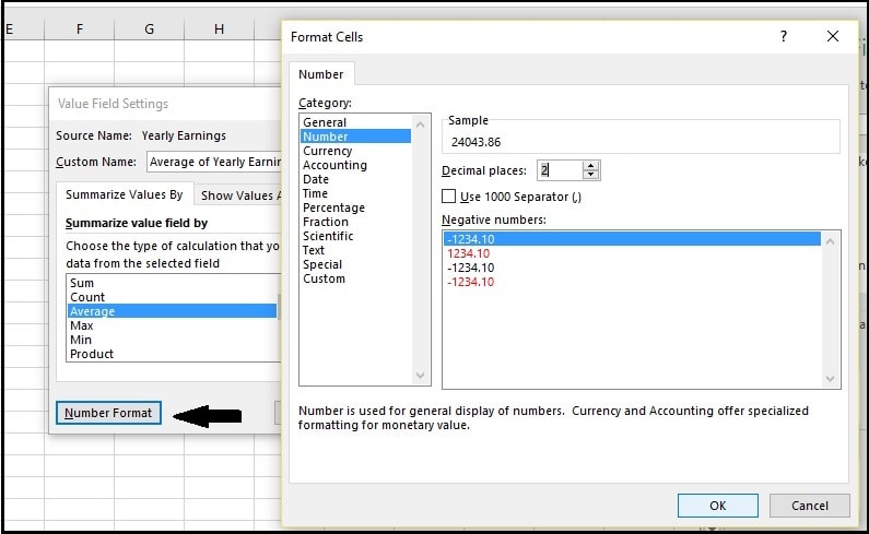
and number format can also be changed.

 

 

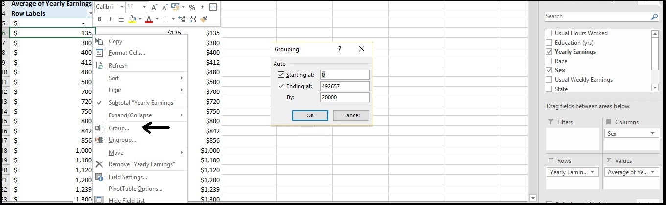
Grouping the values

Now place Sex in columns, Yearly Earnings in Rows and Yearly Earnings in Values. Right click on any of the values and click on Group. A Grouping window will appear where you can select the increment value and click OK.

 

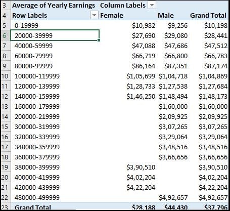
The grouping outcome will look like.

 

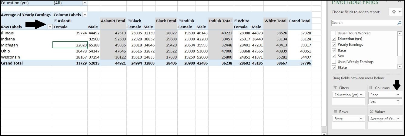
Some more

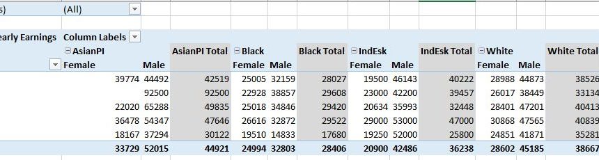
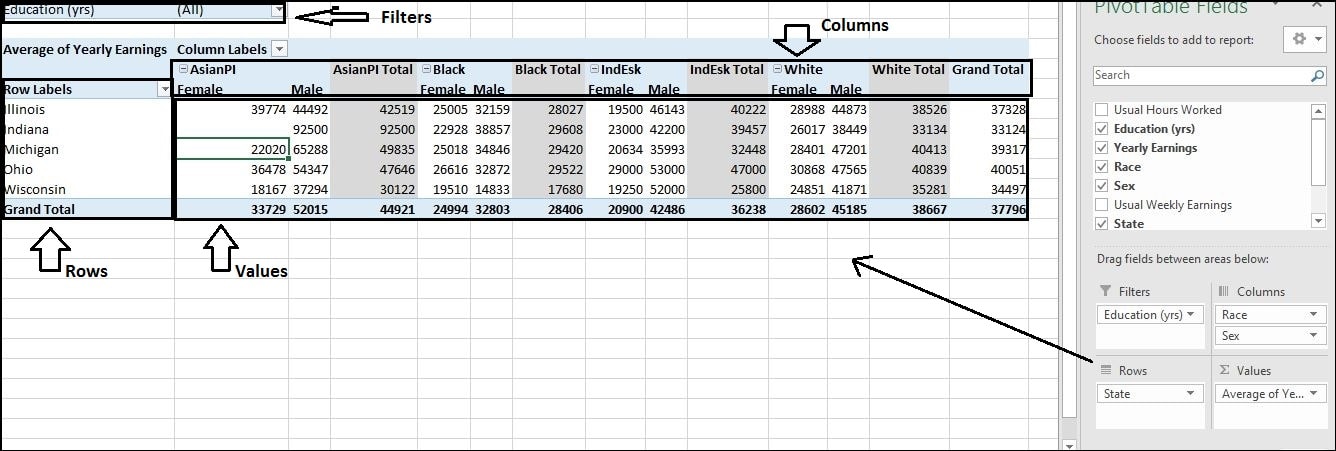
You can add multiple fields in Columns,Rows etc. Here Race and Sex is added to columns. As you can see in the image that both Race and Sex is added to columns.

 

Download worksheet

 

I”ll add more about the Pivot Table till then keep visiting Analytics Tuts for more tutorials.