VLOOKUP and HLOOKUP functions in Excel

July 16, 2016 Niket Kedia Leave a comment

Today we’ll be learning about the one of most important functions in Excel that VLOOKUP and HLOOKUP.

VLOOKUP

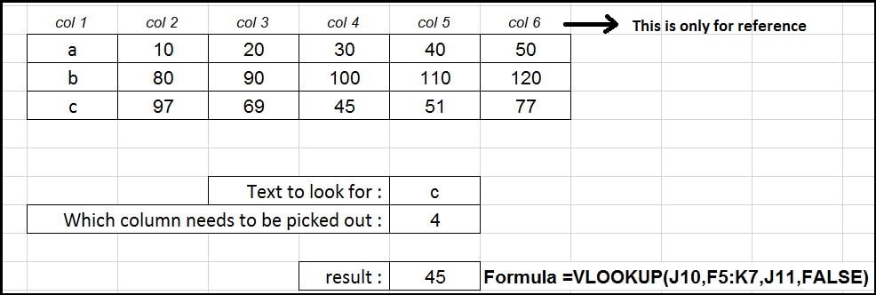
So VLOOKUP or Vertical Lookup works as first Vertical then Horizontal. This function scans down the row headings at the side of a table to find a specified item. When the item is found, it then scans across to pick a cell entry, means it shows below

The formula is as follows:

=VLOOKUP(Item To Find,Range To Look,Column To Pick From,TRUE or FALSE)
*The Item To Find, is a single item specified by the user.
*The Range To Look, is the range of data with the row headings at the left hand side.
*The Column To Pick From, is how far across the table the function should look 
to pick from.
*TRUE for approximate match, FALSE for exact match.

Lets check the example:

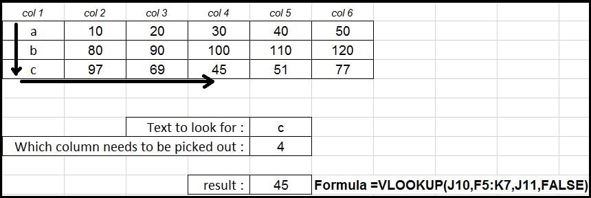
In the image below we can the row headings are a,b,c. According to the formula, we are searching for row heading ‘c’ and column is (including the row heading column) 4. In the range we must consider the row heading column otherwise the formula wont work and the row heading column is the column 1.
So the formula will find the ‘c’ first and then will go to the column 4th. So, the result is 45.

VLOOKUP with TRUE condition

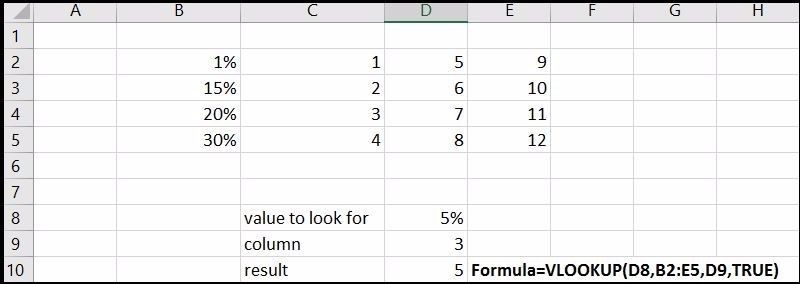
TRUE condition in VLOOKUP will first check for the exact match if that doesn’t match then it take the value below the exact match.
In the example below we are searching for 5% which is not present in the table so it goes
for 1% and the value of the 3rd column is 5 (result).

VLOOKUP with MATCH function

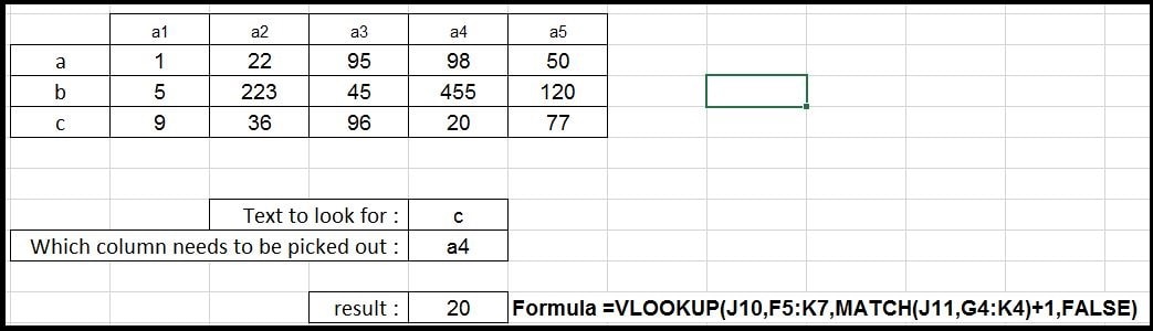
VLOOKUP with MATCH function is also very common method for data handling in excel. Here we can in the image below that, row headings are a,b,c and column headings are a1,a2 and so on. We have done nothing special only getting the column number using the MATCH function. MATCH function returns the position of the item we are searching for.We are searching for ‘a4’ from the column heading that is position 4 but the position in VLOOKUP is 5 that’s why we have added 1 and that is done.

HLOOKUP

HLOOKUP or Horizontal Lookup works as first horizontal then vertical down. This function scans across the column headings at the top of a table to find a specified item. When the item is found, it then scans down the column to pick a cell entry.

The formula is as follows:

=HLOOKUP(Item To Find,Range To Look,Row To Pick From,TRUE or FALSE)
*The Item To Find, is a single item specified by the user.
*The Range To Look, is the range of data with the column headings at the top.
*The RowToPickFrom, is how far down the column the function should look to pick from.
*TRUE for approximate match, FALSE for exact match.

Lets check the example:

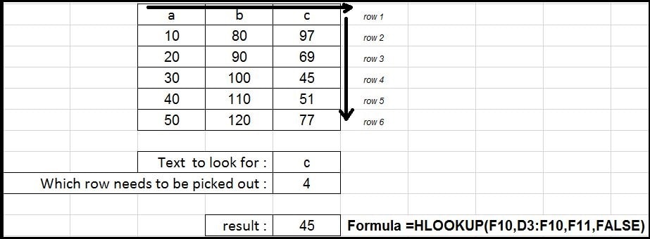
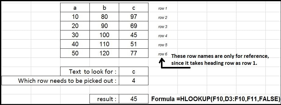
In the image below we can the column headings are a,b,c. According to the formula, we are searching for column heading ‘c’ and row is (including the column heading column) 4. In the range we must consider the column heading row otherwise the formula wont work and the column heading row is the column 1.
So the formula will find the ‘c’ first and then will go to the row 4th. So, the result is 45.

HLOOKUP with TRUE condition

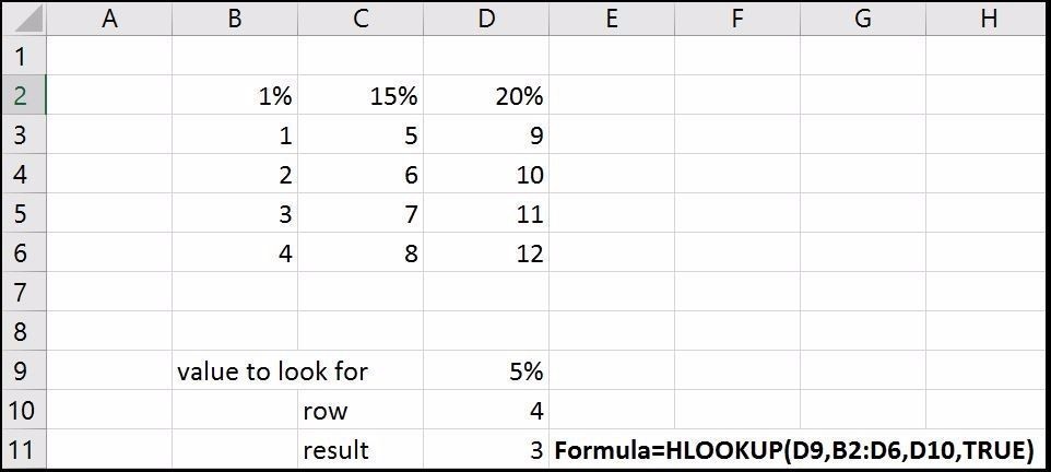
TRUE condition in HLOOKUP will first check for the exact match if that doesn’t matches then it take the value below the exact match.
In the example below we are searching for 5% which is not present in the table so it goes
for 1% and the value of the 4th row is 3 (result).

HLOOKUP with MATCH function

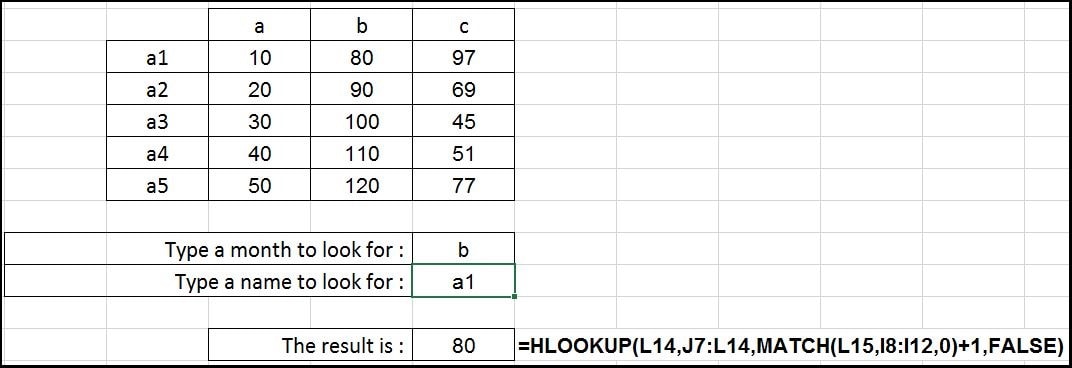
HLOOKUP with MATCH is same as VLOOKUP with MATCH but for row. You can see in the image below.

So this was about the one of the most powerful functions in excel. Comment if you have any doubts

Thanks for reading and keep visiting Analytics Tuts for more tutorials.

Excel